Data transformations with TensorFlow

In this post I will work on the CIFAR-10 dataset, collected by Alex Krizhevsky, Vinod Nair, and Geoffrey Hinton. The images can be downloaded here. Also, find my python notebook(.ipynb) here.

Dataset

First, let’s talk a bit about how our dataset looks like. From the downloading source, we are provided with five training batches and one test batch, each with 10000 randomly-selected images from each class.

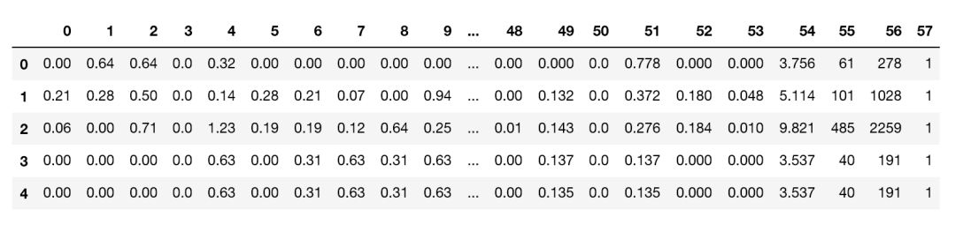
A quick glimpse over the dataset gives us this:

Transformations

Tensorflow might not be the most Deep Learning framework to work with. For this reason, in this blog post I will present a solution using TensorFlow eager execution. For more details, read here.

So, Transformations. Why do we need them? Deep learning models are known to be especially effective and produce very good results. Though, one downside is that they are usually very data hungry. Therefore, given that we have too little data, we apply data transformation over them, and use them in training.

Now, let’s get our hands dirty. “Talk is cheap, show me some code!” (Linus Torvalds)

First, we provide ourselves with all the imports needed:

import tensorflow as tf
import pickle
import pandas as pd
from sklearn.model_selection import train_test_split
from keras.preprocessing.image import ImageDataGenerator
from keras.datasets import cifar10
import numpy as np
import math
import matplotlib.pyplot as plt

For ease of work we enable eager execution.

tf.enable_eager_execution()

Now, we use the [1] implementation to load the dataset.

X_data1, y_data1 = load_cfar10_batch("cifar-10-batches-py", 1) # load the dataset
X_data2, y_data2 = load_cfar10_batch("cifar-10-batches-py", 2) # load the dataset
X_data3, y_data3 = load_cfar10_batch("cifar-10-batches-py", 3) # load the dataset
X_data4, y_data4 = load_cfar10_batch("cifar-10-batches-py", 4) # load the dataset
X_data5, y_data5 = load_cfar10_batch("cifar-10-batches-py", 5) # load the dataset

X_data = np.concatenate((X_data1, X_data2, X_data3, X_data4, X_data5), axis=0)
y_data = np.concatenate((y_data1, y_data2, y_data3, y_data4, y_data5), axis=0)

y_data = tf.Variable(pd.get_dummies(y_data).values) # hot-encode categorical

Next, we create a function to nicely display the original image and its transformations.

def show_image(original_image,translated, cropped_resized, transformed, title="Data transformations"):
    fig=plt.figure()
    fig.suptitle(title)

    original_plt=fig.add_subplot(1,4,1)
    original_plt.set_title('original')
    original_plt.imshow(original_image)

    transformed_plt=fig.add_subplot(1,4,2) 
    transformed_plt.set_title('transformed')
    transformed_plt.imshow(transformed)

    cropped_resized_plt=fig.add_subplot(1,4,3) 
    cropped_resized_plt.set_title('rescaled')
    cropped_resized_plt.imshow(cropped_resized)

    translated_plt=fig.add_subplot(1,4,4) 
    translated_plt.set_title('translated')
    translated_plt.imshow(translated)

    plt.show(block=True)

Data Transform

We now apply the three transformations and merge everything in a bigger data array. We also take into account the size of the labels dataset.

data = X_data
label = y_data

translated = tf.cast(tf.contrib.image.translate(data, translations=[5, 5]), dtype=tf.uint8)
cropped_resized = tf.cast(tf.image.crop_and_resize(data, boxes=[[0.0, 0.0, 0.89, 0.89]]*X_data.shape[0], crop_size = [32, 32], box_ind=np.arange(X_data.shape[0])), dtype=tf.uint8)
transformed = tf.cast(tf.contrib.image.transform(data, [1, tf.sin(-0.2), 0, 0, tf.cos(-0.2), 0, 0, 0]), dtype=tf.uint8)

merged = tf.concat([data, translated, cropped_resized, transformed], axis=0)
labels = tf.concat([label, label, label, label], axis=0)

Visually, a transformed images look as follows:

show_image(data[42], translated[42], cropped_resized[42], transformed[42])

Data Split into train and test

We use train_test_split from sklearn over the transformed dataset. We return training and testing samples and then we pickle them for future use.

X_train, X_test, y_train, y_test = train_test_split(np.array(merged), np.array(labels), test_size=0.33, random_state=42)

And, because we want to use that in future, let us save transformed data in a pickle file.

output = open('data.pkl', 'wb')
pickle.dump(((X_train, y_train), (X_test, y_test)), output)

Was quite a long way till now. But we did it! Hooray! 😁  Although it is not a complicated stuff, it took me quite a while to play with it. For this reason, I decided to share it with the world. Also, find the python notebook(.ipynb) here.

References

1. https://towardsdatascience.com/cifar-10-image-classification-in-tensorflow-5b501f7dc77c, accessed online June 23rd, 2010

mpi4py – how it works

Message passing interfaces are a powerful tool for parallelizing problems by dividing them in subtasks, and therefore achieving better performance results in terms of time. When Init(args) is called, the MPI system is being initialised.

The underlying principle of MPI intercommunication is based on a concept called communicator. A ​communicator defines a group of processes. Group membership means that processes are able to communicate with each other. Such a communicator could be ​COMM_WORLD​. This is the default Intracommunicator, but one could play around customising different types of communicators. In order to be able to work with these processes one needs to know how to identify them i.e. how does a process know who he is or how many processes are out there. For this scope a unique ID called ​rank is assigned to each process, and a process can address himself other processes by using this rank.

One could address to the communicator to get its own rank: getRank()​. The communication between processes happens through ​send() and operations. To identify a message uniquely the sender will provide the message with a tag.

Then the receiver will handle the message accordingly. Such a communication is known as ​point-to-point communication.

One might be also interested in involving multiple processes and there is where collective communication comes into play. ​Collective communication is an advanced functionality that enables multiple processes to communicate with each other by sharing messages in a complex fashion, such as broadcasting, scattering, gathering, etc.

Graphically, the way MPI works is as follows:

 

Spam filter using libsvm

In this post we are going to have a quick look at libsvm and do a basic classification on spam vs not spam email.

We will use this SpamBase dataset, which you can download yourself here. The dataset contains features such as word and character frequency, which you can find in the dataset description.

In order to use the libsvm for classification we need, and that is the main aim of this post, to convert the dataset to libsvm format, that is < label > < index1 >:< value1 > < index2 >:< value2 >. . .

So let us proceed to the actual implementation. We first do the imports:

import matplotlib.pyplot as plt
from svmutil import *
import pandas as pd
import numpy as np

Next we load the dataset using pandas. For libsvm we actually do not need to know the feature names, because the feature are labels sth like 1:value, 2: value, 3:value, etc…

data = pd.read_csv("../../data/spambase.data", sep=",", header=None)
data.head()

 

This produces the following output:

Let’s convert dataset into a libsvm format. Since the targets should be in the following column we take this into account in the following python func:

def format(dataframe, file_name):
    f = open(file_name, 'w')

    for index, row in dataframe.iterrows():
        line = ""
        line += str(int(row[57]))
        for col in list(dataframe)[:-1]:
            line += " " + str(col+1) + ":" + str(row[col])
            line += "\n"
        f.write(line)

    f.close()

proportion = 0.8
rand_select = np.random.rand(len(data)) <= proportion
format(data[rand_select], "train.txt")
format(data[~rand_select], "test.txt")

We now split the data to train and test:

y_train, X_train = svm_read_problem('train.txt')
y_test, X_test = svm_read_problem('test.txt')

Now let’s do a grid search over parameter C:

C = [0.01, 0.1, 1, 10, 100]
training_options = []

for c in C:
    training_options.append("-c " + str(c))

We train for each of the C values:

prob = svm_problem(y_train, X_train)
models = []

for param in training_options:
    models.append(svm_train(prob, param))

We now test on the model to see how it performed:

useScipy = True
test_performance = []
train_performance = []
for model in models:
    p_labels, p_acc, p_vals = svm_predict(y_test, X_test, model)
    test_performance.append(evaluations(y_test, p_labels, useScipy))
    p_labels, p_acc, p_vals = svm_predict(y_train, X_train, model)
    train_performance.append(evaluations(y_train, p_labels, useScipy))

Let’s construct the lists of performances on both train and test dataset so that we could easily plot them:

test_accuracies = []
train_accuracies = []

for i in range(len(test_performance)):
    test_accuracies.append(test_performance[i][0])
    train_accuracies.append(train_performance[i][0])

Now, let’s visualize them:

fig, axs = plt.subplots(1, 1, figsize=(25, 10))
fig.suptitle("Accuracy vs C values")
axs.plot(C, test_accuracies, label="Test")
axs.plot(C, test_accuracies, "o")
axs.plot(C, train_accuracies, label="Train")
axs.plot(C, train_accuracies, "o")
axs.legend()
plt.show()

This produced the following output:

Seems like some c value close to 10 is the most suitable on both the train and test set. Naturally, we also notice that the accuracy is better on train dataset, which is usually a normal behavior, since it has already seen this data.

Libsvm is surely a great library, though to get a better view of it one should experience himself with it, so don’t miss the opportunity to get your hands a bit dirty and go for some code. 😉

Tree Traversals

In this post we are going to take a look at in-order, pre-order and post-order tree-traversals implementations in Java.

First, what is a tree traversal?

According to Wikipedia[1], a tree traversal (also known as tree search) is a form of graph traversal and refers to the process of visiting (checking and/or updating) each node in a tree data structure, exactly once.

InOrder – having a node n visits: left node of node n, then n itself, then right node of n.

PreOrder – having a node n visits: n itself, then left node of node n , then right node of n.

PostOrder – having a node n visits: left node of node n , then right node of n, then n itself.

Let’s write the code for Tree Traversal class:

import java.util.ArrayList;
import java.util.List;

public class TreeTraversal {

    private List visitednodesInorder = new ArrayList();
    private List visitednodesPreorder = new ArrayList();
    private List visitedNodesPostorder = new ArrayList();

    public List inOrderTraversal(Node node) {
        if (node != null) {
            inOrderTraversal(node.getLeft());

            node.visit();

            visitednodesInorder.add((char)node.getContent());

            inOrderTraversal(node.getRight());
         }
         return visitednodesInorder;
    }

    public List preOrderTraversal(Node node) {
        if (node != null) {
            node.visit();

            visitednodesPreorder.add((char)node.getContent());

            preOrderTraversal(node.getLeft());
            preOrderTraversal(node.getRight());
        }
        return visitednodesPreorder;
    }

    public List postOrderTraversal(Node node) {
        if (node != null) {
            postOrderTraversal(node.getLeft());
            postOrderTraversal(node.getRight());

            node.visit();
            visitedNodesPostorder.add((char)node.getContent());
        }
        return visitedNodesPostorder;
    }
}

Now let us see it in action:

import org.junit.jupiter.api.BeforeEach;
import org.junit.jupiter.api.Test;

import java.util.ArrayList;
import java.util.List;

import static org.junit.jupiter.api.Assertions.assertEquals;

public class TraversalTest {
    private static Node root;

    private static TreeTraversal traversal;

    @Test
    public  void inOrderTraversalTest() {
        List<Character> traversedNodes = traversal.inOrderTraversal(root);
        List<Character> expected = new ArrayList<Character>();
        expected.add('d'); expected.add('o'); expected.add('e'); expected.add('a');
        expected.add('f'); expected.add('p'); expected.add('g');

        assertEquals(traversedNodes, expected);
    }

    @Test
    public void preOrderTraversalTest() {
        List<Character> traversedNodes = traversal.preOrderTraversal(root);
        List<Character> expected = new ArrayList<Character>();
        expected.add('a'); expected.add('o'); expected.add('d'); expected.add('e');
        expected.add('p'); expected.add('f'); expected.add('g');

        assertEquals(expected, traversedNodes);
    }

    @Test
    public void postOrderTraversalTest() {
        List<Character> traversedNodes = traversal.postOrderTraversal(root);
        List<Character> expected = new ArrayList<Character>();
        expected.add('d'); expected.add('e'); expected.add('o'); expected.add('f');
        expected.add('g'); expected.add('p'); expected.add('a');

        assertEquals(expected, traversedNodes);
    }

    @BeforeEach
    public void setup()  {
        // build the tree
        root = new Node();
        root.setContent('a');

        Node leftChild1 = new Node();
        leftChild1.setContent('o');

        Node rightChild1 = new Node();
        rightChild1.setContent('p');

        root.setLeft(leftChild1);
        root.setRight(rightChild1);

        // building left child on level one
        Node leftChild2 = new Node();
        leftChild2.setContent('d');

        Node rightChild2 = new Node();
        rightChild2.setContent('e');

        leftChild1.setLeft(leftChild2);
        leftChild1.setRight(rightChild2);

        // building right child on level one
        Node lfetChild3 = new Node();
        lfetChild3.setContent('f');

        Node rightChild3 = new Node();
        rightChild3.setContent('g');

        rightChild1.setLeft(lfetChild3);
        rightChild1.setRight(rightChild3);

        traversal = new TreeTraversal();
    }
}

Also, keep in mind the class for Node:

public class Node {
    private Node parent;
    private Node left;
    private Node right;

    private char content;

    private boolean isVisetd;

    public void visit() {
        this.isVisetd = true;
    }

    public Node() {
    }

    public Node getLeft() {
        return left;
    }

    public void setLeft(Node left) {
        this.left = left;
    }

    public Node getRight() {
        return right;
    }

    public void setRight(Node right) {
        this.right = right;
    }

    public int getContent() {
        return content;
    }

    public void setContent(char content) {
        this.content = content;
    }

}

Finally all the tests have passed, meaning the implementation was done correctly.

References:

1. https://en.wikipedia.org/wiki/Tree_traversal

MovieLens Dataset Analysis

In this post I take a look at MovieLens Dataset and will do a exhaustive analysis using plotly library.

Before that, let us import all the necessary libraries:

import numpy as np
import pandas as pd
import matplotlib.pyplot as plt
import seaborn as sns
import warnings
import plotly.offline as py
warnings.filterwarnings('ignore')

py.init_notebook_mode(connected=True)
import plotly.graph_objs as go

 

Now let us load the dataset:

import numpy as np

file_path = "data/u.user"
names = ["user_id", "age", "gender", "occupation", "zip_code"]

user_df = pd.read_csv(file_path, names=names, sep="|")
print("Missing values: ", user_df.isnull().values.any())
user_df.head()
 

Let us see who are people by means of gender:

colors = ['#a1a8b5', '#f4cb42'] # bronze, silver
gender_counts = user_df.gender.value_counts(sort=True)
labels = gender_counts.index
values = gender_counts.values pie = go.Pie(labels=labels, values=values, marker=dict(colors=colors))

layout = go.Layout(title='Gender distribution')

fig = go.Figure(data=[pie], layout=layout)
py.iplot(fig) 

 

It looks like women keep themeselves busy with something else, rather than watching movies. ))  What about their age?

men = user_df[user_df.gender=='M'].age
women = user_df[user_df.gender=='F'].age box_m = go.Box(x=men, name="Male", fillcolor='navy')

box_w = go.Box(x=women, name="Female", fillcolor='lime')

layout = go.Layout(title='Age by sex')

fig = go.Figure(data=[box_m, box_w], layout=layout)
py.iplot(fig)

Let us see some information about the users themselves – what is the mean age, how many women/men do we have, who is our audience(occupation):

topn = 10
count_male = male.dropna().occupation.value_counts()[:topn].reset_index()
count_female = female.dropna().occupation.value_counts()[:topn].reset_index()
pie_men = go.Pie(labels=count_male['index'],values=count_male.occupation,name="Men",hole=0.4,domain={'x': [0,0.46]})
pie_women = go.Pie(labels=count_female['index'],values=count_female.occupation,name="Women",hole=0.4,domain={'x': [0.5,1]})

layout = dict(title = 'Top-10 occupations by gender', font=dict(size=15), legend=dict(orientation="h"),

annotations = [dict(x=0.2, y=0.5, text='Men', showarrow=False, font=dict(size=20)),
dict(x=0.8, y=0.5, text='Women', showarrow=False, font=dict(size=20)) ])

fig = dict(data=[pie_men, pie_women], layout=layout)
py.iplot(fig)

Lot’s of students in both men and women. Approx 4% more of female administrators, but no woman executive 😦 . While women artists watch movie, seems men are not. By taking a look at technical occupation categories such as “scientist”, “technician” or “programmer” we could draw a general conclusion, that women are less attracted by technical areas.

And who rates what? Are the movies rated by women and men more or less uniformly?

scatterplots = list()
for movie_id in movie_df.movie_id:
    orth = top_movies_male[top_movies_male['index'] == movie_id].movie_id.values
    vert = top_movies_female[top_movies_female['index'] == movie_id].movie_id.values
    trace = go.Scatter(
        x = orth if orth != None else [0],
        y = vert if vert != None else [0],
        name = movie_df[movie_df.movie_id==movie_id].movie_title.values[0],
        marker=dict(
            symbol='circle',
            sizemode='area',
            sizeref=40)
        )
    scatterplots.append(trace)

layout = go.Layout(title='Men vs Women rating count per movie',
    xaxis=dict(title='Men, nr. ratings'),
    yaxis=dict(title='Women, nr .ratings'),
    showlegend=False)

fig = dict(data = scatterplots, layout = layout)
py.iplot(fig)

As we notice, only a couple of movies are heavily rated. Also, we see that this happens more or less same in men as in women. The line would be described smth as y = 0.5x. And that is legit, since the nr of men is ~ twice as the nr of women.

Software Engineering Internship at Tacit Knowledge

Like it or not, in order to get a job you need working experience. To build it, funny enough, you should first get a job. See the catch 22? In the pursuit of learning stuff and improving my technical skills I performed the Software Engineering Internship at Tacit Knowledge. Frankly, did I learn so many things…

I just happened to be at Tekwill (an ICT excellent build recently in Moldova) – there usually happen a lot of events, and as I do really like to get involved in pretty much everything moving around, I was there doing some meetings. At some point Ana Chirita – the Executive Director or ATIC, and a really bright person who did bring so much impact in the development of the local IT community, suddenly asked me: “Did Tacit Knowledge contact you? I recommended you for their Software Engineering position.” You have no idea how happy I was. Firstly, because wow, I was just did referred by this really powerful woman, and secondly because of Tacit Knowledge – one of the top companies in Moldova. I was definitely excited about the idea. After several weeks I have actually had the Screening interview with the HR, and then I was invited to the interview.

The technical interview went well. It feel it was more challenging than interviews in other companies on the same position – Software Engineering Intern. I would describe the interview as a “friendly technical discussion”, and I felt free to think out loud, and whenever I will get stuck, the interviewers will enhance the process. We went through my CV, discussed my experienced, then have proceeded to more technical questions. What I did like about the technical part, was that I was put in situations to be actually thinking, and to mind edge cases as well. Interviewers will ask tricky questions in order to see whether I have a deep understanding of the discussed concepts. A few days later I received an email, and guess what? Great news – I start February the 5th, 9am!

I did really like the way they organized everything – a laptop was waiting me on my desk, and basically everything was just set up for me to start learning and creating value. The office was really really nice and it just felt so “inviting” to work and focus on your task. And coffee. That’s a must for me! The first two weeks we have passed through an “on-boarding” phase, where we have basically learned more about the company, but meanwhile we have already been given tasks.

One of the greatest things Tacit is good at is enhancing the learning process. We’ve been assigned practical tasks from the very beginning, and were given online resources and books. Those have slightly improved my technical skills, and it’s cool that we were immediately applying them on our pilot project. Nevertheless, I consider the most important and valuable experience of all working on a real project. Here I worked with real employees, on real code, and every change was a well thought decision. Thanks to my very amazing team I have managed to quickly integrate. I did have many questions at the beginning, but people were open to explain. They would also always ask me first how would I solve specific puzzles, so that they will make sure I have foreseen all the edge cases. This I consider to be a better approach than just telling interns the solution. This way I learned much more. Because people are highly experienced, Tacit taught me to be mindful about code quality, which is a top priority for long-term projects.

I’m grateful to have had the opportunity to be part of TK team. Tacit taught me a lot of things, both technical and soft. Besides the professional environment, coding techniques and habits, technologies, project phases, development lifecycle and methodologies, the culture of Tacit made me value things like consistent learning and understanding, the will of self improvement and common value creation. It’s amazing to see each member’s dedication and initiative in the improvement of projects, processes, code quality, and as a result – products. This is probably the first thing to be checked before anyone is being considered for a position at Tacit.